Image Generation with Generative Adversarial Networks (GAN)
Introduction
In this article, I implemented some variants of DCGAN[1], which is one of the generative adversarial networks. The DCGAN model has replaced the fully connected layer with the global pooling layer. It is universally acknowledged that the purpose of GAN is to achieve Nash equilibrium between the discriminator and the generator. That is to say, neither of these two models should perform very well. When I applied the DCGAN to dataset CUB200-2011, I find that the loss of the generator converges to zero rapidly while the loss of the discriminator stays high, which shows that the discriminator can not distinguish the fake images from all images in this case. To improve its performance, I add a fully connected layer at the end of the convolution layer in the discriminator. The outcome is better than the original DCGAN.
Codes
main.py
1 | |
DCGAN.py
1 | |
Results
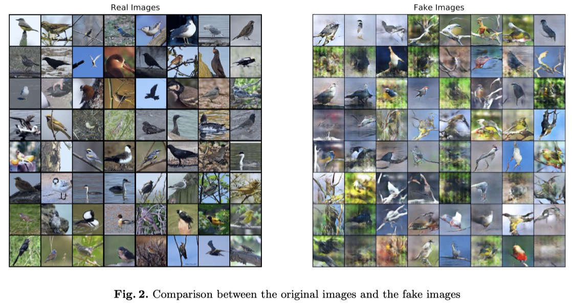
The generated images compared to the original images are shown as follows. The left grid contains the real ones, the right images are fake.

It can be observed that the fake images are close to the real images, and even some of the generated images are difficult for people to distinguish from real ones. Of course, some images are slightly blurred with green backgrounds.
In order to see the evolution of the generated images, I also visualize these fake images at different epochs. It is interesting to see that some latent features have been extracted at the early stage. At the 50th iteration, the whole birds’ outlines have begun to appear.

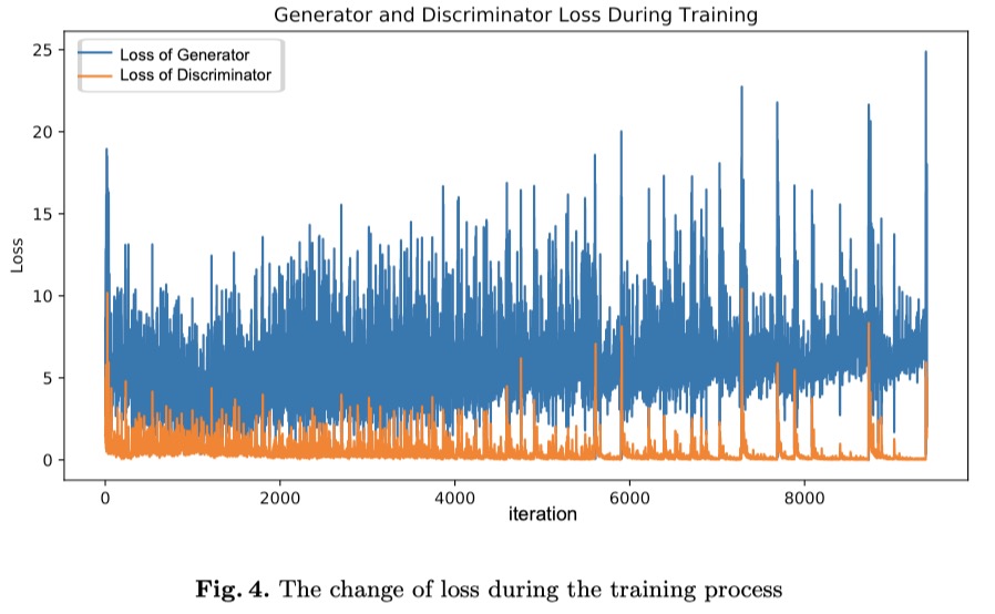
The following figure shows the change of loss during the training process. We can see that the loss of the generator is a little higher than that of the discriminator. One of the possible reasons is the existence of the fully connected layer. We can also see the losses are not steady for both of them, which may lead to the mode collapse.

Feature Visualization
In this part, I visualize the attention of different intermediate layers of discriminator in DCGAN with the help of Grad-CAM[2]. Grad-CAM uses the gradient information of the last convolution layer flowing into CNN to assign important values to each neuron. Specifically, the gradient of class is calculated by using (Logits before softmax), and the activation value of the feature graph is defined as . These backflow gradients are applied with the global pooling strategy on the width and height dimensions (indexed by and , respectively) to obtain neuron importance Iights . Equation 1 and 2 describes the process.
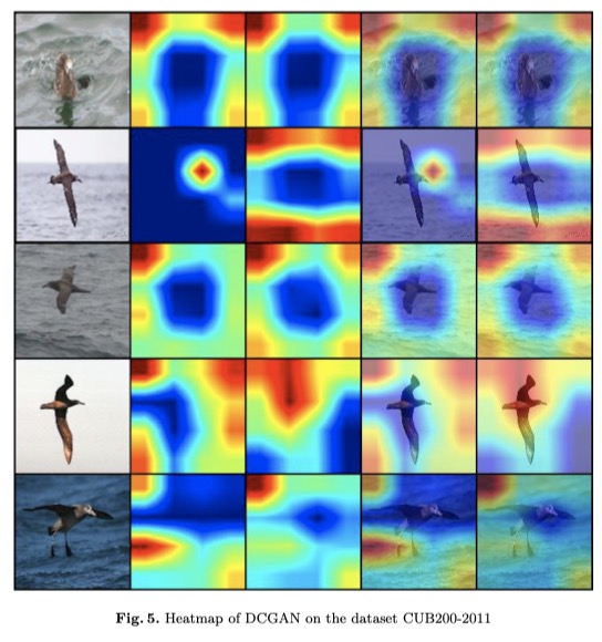
The heatmap of the last convolutional layer of discriminator in DCGAN in the case of dataset CUB200-2011 is shown as follows. The second and third columns are heatmaps of Grad-CAM and Grad-CAM++[3] respectively. The last two columns are the results superimposed on the original images. I choose to visualize the attention that makes the discriminator judge fake. As can be seen from the results, the place with higher heat value is not birds, but the environment in most cases, which valids that the discriminator should not perform so ill in GAN model.

[1] Radford, Alec, Luke Metz, and Soumith Chintala. “Unsupervised representation learning with deep convolutional generative adversarial networks.” arXiv preprint arXiv:1511.06434 (2015).
[2] Selvaraju, Ramprasaath R., et al. “Grad-cam: Visual explanations from deep networks via gradient-based localization.” Proceedings of the IEEE international conference on computer vision. 2017.
[3] Chattopadhay, Aditya, et al. “Grad-cam++: Generalized gradient-based visual explanations for deep convolutional networks.” 2018 IEEE Winter Conference on Applications of Computer Vision (WACV). IEEE, 2018.
OmegaXYZ.com
All rights reserved.
OmegaXYZ is licensed under a CC BY-SA 4.0 Generic License.